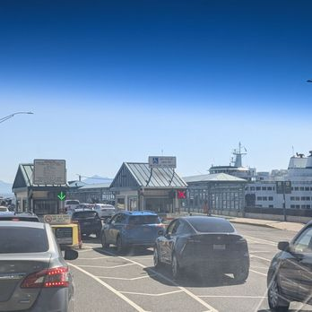
Cars lined up at the ferry toll booths, with a boat waiting at the dock. Photo: Davin Fladager-McCullough.
Class topic: MATH& 146, Sections 4.1–4.3 — scatter diagrams, correlation, the least-squares regression line, residuals, the coefficient of determination (R²) and influential observations.
On a summer afternoon at Mukilteo, the car lanes fill up and the boat leaves late. It’s easy to connect the two: a full boat takes longer to load, so a full boat must be a late boat.
That’s a claim about two numbers moving together, and my class just covered how to measure that. So I asked: do fuller ferries leave later? And if they do, how much of the lateness does the crowd actually explain?
The answer: yes, fuller boats leave later. But the crowd explains less than I expected, and something else explains about twice as much.
Where the numbers come from
Washington State Ferries records two things for every sailing on my route, and posts both on its public dashboard:1
Minutes late: how long after the scheduled time the boat actually left. The boats carry transponders, and a system matches each departure to the schedule.
Cars through the toll booth: how many vehicles paid at the terminal between the previous sailing and this one.
That second number is not the same as cars on the boat. It counts cars that paid, not cars that got on. On a busy day some of those cars wait for the next boat. I used the booth count anyway because it’s the best measure of “how crowded” WSF publishes per sailing.
I downloaded every sailing for an earlier post. For this one I kept summer 2025 (June–August), the latest full summer in the data. That leaves 6,365 sailings that have both a delay and a booth count.
This isn’t a sample. It’s every recorded sailing that summer, so there’s no margin of error. The limits come from what the system records, and I flag them as they come up.
What I did in R
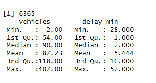
My summer 2025 sailings in R: how many there are, and the range of cars and minutes late.
Show the code
sailings <-read.csv("../2026-09-28-ferry-runs-late/muk-clinton-sailings.csv")# Summer 2025 (June-August), sailings with both a recorded delay and a toll-booth countsummer <-subset(sailings, year ==2025& month %in%6:8&!is.na(delay_min) &!is.na(vehicles))nrow(summer)
[1] 6365
Show the code
summary(summer[, c("vehicles", "delay_min")])
    vehicles        delay_min
 Min.   :  2.00   Min.   :-28.000
 1st Qu.: 54.00   1st Qu.:  1.000
 Median : 90.00   Median :  2.000
 Mean   : 87.23   Mean   :  5.444
 3rd Qu.:118.00   3rd Qu.: 10.000
 Max.   :407.00   Max.   : 52.000
A typical sailing that summer had 90 cars through the booth and left 2 minutes late (those are the medians). The boats on this route carry 124 or 144 cars, depending on which boat is running.
When I compare two numbers like this, my class calls them the explanatory variable (the one I think does the pushing: cars) and the response variable (the one that might respond: minutes late). The explanatory variable goes on the horizontal axis.
Yes, fuller boats leave later
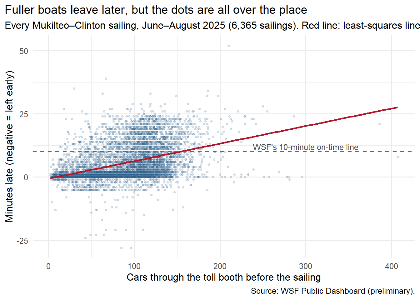
A scatter diagram puts one dot on the chart for each sailing: across for cars, up for minutes late.
Show the code
library(ggplot2)ggplot(summer, aes(x = vehicles, y = delay_min)) +geom_point(alpha =0.15, size =0.9, colour ="#2c5f8a") +geom_smooth(method ="lm", formula = y ~ x, se =FALSE, colour ="#b2182b", linewidth =1) +geom_hline(yintercept =10, linetype ="dashed", colour ="grey40") +annotate("text", x =300, y =12, label ="WSF's 10-minute on-time line", size =3.4, colour ="grey30") +labs(x ="Cars through the toll booth before the sailing", y ="Minutes late (negative = left early)",title ="Fuller boats leave later, but the dots are all over the place",subtitle ="Every Mukilteo–Clinton sailing, June–August 2025 (6,365 sailings). Red line: least-squares line.",caption ="Source: WSF Public Dashboard (preliminary).") +theme_minimal(base_size =12) +theme(plot.title.position ="plot")
The cloud tilts up. Boats with few cars almost always left on time. Boats with lots of cars sometimes left on time and sometimes left very late.
The correlation coefficient, r, puts a number on that tilt. It runs from −1 to 1. Near 1 means the dots hug a rising straight line, near −1 a falling one, near 0 no straight-line pattern at all.
Show the code
n <-nrow(summer)r <-cor(summer$vehicles, summer$delay_min)# Critical value for r at this sample size (the same test as the textbook's table, 5% level)t_crit <-qt(0.975, df = n -2)r_crit <- t_crit /sqrt(n -2+ t_crit^2)round(c(n = n, r = r, critical_value = r_crit), 3)
             n              r critical_value
      6365.000          0.414          0.025
My correlation in R: 6,365 sailings, r = 0.414, and the critical value for that many sailings, 0.025.
r = 0.41. That’s a positive relationship, but a loose one.
My class tests an r against a critical value: if r is bigger than the critical value, the straight-line relationship is probably not a fluke. The textbook’s table stops at 30 data points, where the critical value is 0.361. With 6,365 sailings, it shrinks to 0.025.2 My r of 0.41 clears that easily.
That’s worth slowing down on. With this much data, almost any relationship clears the bar. Passing the test means “this isn’t chance.” It does not mean “this is strong.” For strength, I need the next two tools.
Each extra car costs about 4 seconds
The red line on the chart is the least-squares regression line: the one straight line that comes closest to all the dots at once. (“Closest” has a precise meaning: it makes the total of the squared up-and-down misses as small as possible.)
Show the code
cars_line <-lm(delay_min ~ vehicles, data = summer) # least-squares line: minutes late from carscoef(cars_line) # intercept and slope
(Intercept)    vehicles
 -0.6081367   0.0693868
Show the code
summary(cars_line)$r.squared # R-squared
[1] 0.1712653
Show the code
predict(cars_line, data.frame(vehicles =c(44, 90, 144))) # light, typical and full boat
       1        2        3
2.444883 5.636676 9.383563
The line is:
predicted minutes late = −0.61 + 0.069 × cars
The slope, 0.069, is the story. Each extra car through the booth goes with about 0.069 more minutes late. That’s about 4 seconds a car, or about 7 minutes per 100 cars.
Cars through the booth
Predicted minutes late
44 (a light sailing)
2.4
90 (typical)
5.6
144 (a full big boat)
9.4
The intercept, −0.61, is what the line predicts for zero cars: leaving about half a minute early. That doesn’t mean anything real. Boats don’t leave early on purpose, and hardly any sailing had close to zero cars. The intercept is just where the line has to start so the slope fits the data.
The crowd explains 17%
The coefficient of determination, R², answers “how much of the up-and-down in minutes late lines up with cars?” For a single straight line it’s just r squared: 0.41 × 0.41 ≈ 0.17.
R² = 0.17. Cars explain about 17% of the variation in how late summer sailings left. The other 83% is everything else: weather, tides, a slow car on the ramp, a crew shortage, a boat that was already running late.
So the crowd matters, but it’s a small part of the story.
Full boats are harder to predict
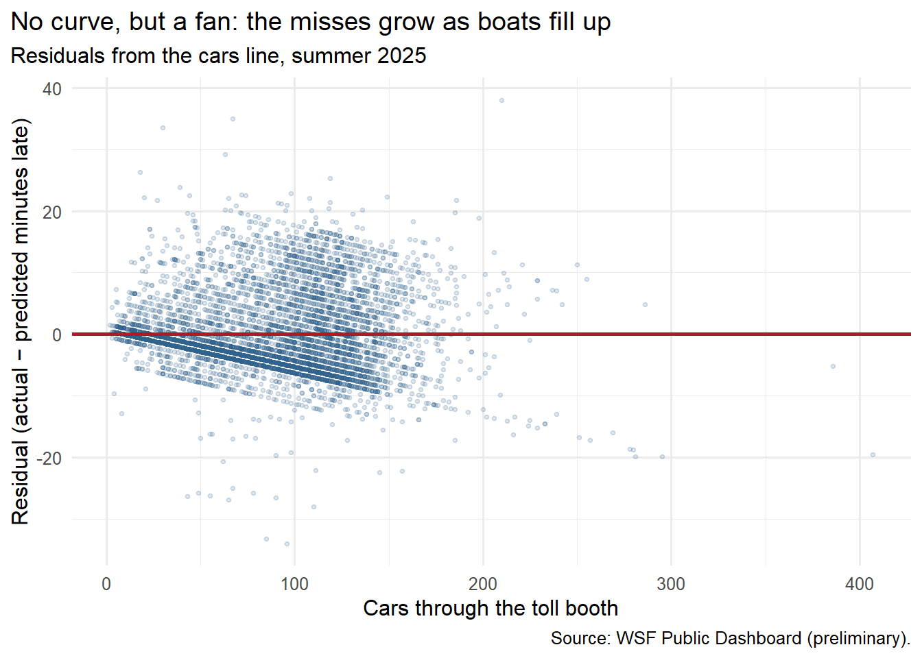
A residual is how far one sailing landed from the line: actual minutes late minus predicted. A positive residual means the boat left later than the line expected. A residual plot charts those misses against cars. If a straight line is the right shape, the dots should scatter evenly around zero, with no curve and no fan.
Show the code
summer$residual <-resid(cars_line) # actual minus predictedggplot(summer, aes(x = vehicles, y = residual)) +geom_point(alpha =0.15, size =0.9, colour ="#2c5f8a") +geom_hline(yintercept =0, colour ="#b2182b", linewidth =1) +labs(x ="Cars through the toll booth", y ="Residual (actual − predicted minutes late)",title ="No curve, but a fan: the misses grow as boats fill up",subtitle ="Residuals from the cars line, summer 2025",caption ="Source: WSF Public Dashboard (preliminary).") +theme_minimal(base_size =12) +theme(plot.title.position ="plot")
The sharp edge along the bottom of the plot is the many sailings that left right on time. A boat can’t leave much earlier than scheduled, so for an on-time sailing the miss is just the line’s prediction with a minus sign, and that edge slopes down as the prediction rises.
Two things show up. First, the average miss stays near zero for every group: no curve, so a straight line is a fair summary of the trend. Second, the misses fan out. For light sailings the line is usually within about 4 minutes. For the busiest sailings the typical miss is almost 10 minutes.
So the line’s “9.4 minutes late for a full boat” is an average with a lot of wiggle. A full boat might leave on time or half an hour late.
Do a few weird sailings drive the line?
An influential observation is a single data point that changes the line a lot when you take it out. My homework had examples where one point out of six flipped the whole answer.
Six sailings in my data look strange: more than twice as many cars through the booth as the boat can carry, up to 407 cars for a 144-car boat. My guess is the counting window stretched over a canceled or skipped sailing, so two boatloads of cars got credited to one departure. I can’t confirm that from the data.
Show the code
odd <- summer$vehicles >2* summer$vehicle_capacity # more than two boatloads through the boothsummer[odd, c("date", "direction", "time", "vessel", "vehicles", "delay_min")]
             date     direction  time    vessel vehicles delay_min
140355 2025-06-12 From Mukilteo 20:35    Kitsap      280         0
142846 2025-07-16 From Mukilteo 13:30    Kitsap      281        -1
142934 2025-07-17 From Mukilteo 21:00    Kitsap      295         0
143046 2025-07-19  From Clinton 20:00   Tokitae      407         8
143115 2025-07-20  From Clinton 17:35    Kitsap      255        26
146226 2025-08-31  From Clinton 21:00 Suquamish      386        21
          (Intercept) vehicles
all           -0.6081   0.0694
without_6     -0.7342   0.0710
Taking them out moves the slope from 0.0694 to 0.0710. Hardly anything. With 6,365 sailings, six odd ones can’t push the line around. That’s the upside of lots of data: no single sailing is influential here.
The hidden third number: time of day
My class warns that a correlation can come from a lurking variable: a third thing that drives both numbers. On this route, time of day is an obvious suspect. Afternoons bring the most cars and the most delays. So maybe cars and lateness move together partly because both follow the clock.
I split the summer into three parts of the day and looked inside each.
             sailings avg_cars avg_min_late    r slope
Before 10 am     2006       72          1.3 0.29 0.018
10 am - 7 pm     3005      109          8.5 0.36 0.087
After 7 pm       1354       62          4.8 0.30 0.048
Part of day
Sailings
Average cars
Average minutes late
r
Slope (min per car)
Before 10 a.m.
2,006
72
1.3
0.29
0.018
10 a.m. – 7 p.m.
3,005
109
8.5
0.36
0.087
After 7 p.m.
1,354
62
4.8
0.30
0.048
Time of day is part of it. Midday and afternoon sailings had the most cars and ran the latest, and inside each part of the day r drops below the overall 0.41.
But cars still matter within each part of the day. And the slope changes a lot. Before 10 a.m., 100 extra cars go with less than 2 extra minutes. Between 10 and 7, the same 100 cars go with almost 9. A crowd costs more on a boat that’s already behind schedule. That points to the bigger story.
What really predicts my boat: its last trip
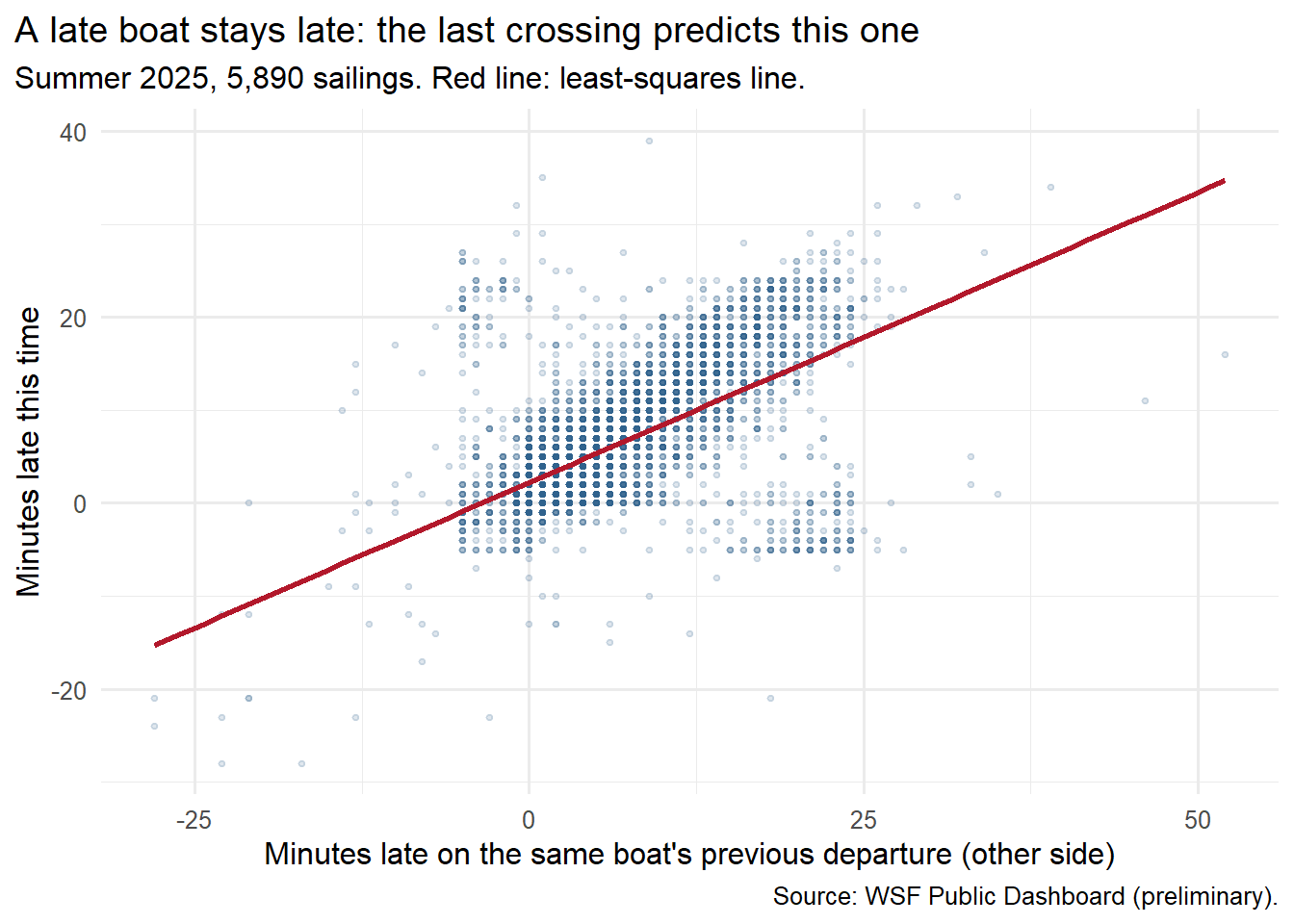
A ferry can’t leave Mukilteo until it gets there from Clinton. So I tried a different explanatory variable: how late the same boat left the other side on its previous crossing, usually about 30 minutes earlier.
Show the code
# For each boat on each day, find how late its previous departure (from the other terminal) wassailings <- sailings[order(sailings$date, sailings$vessel, sailings$clock_min), ]boat_day <-paste(sailings$date, sailings$vessel)sailings$prev_leg_delay <-ave(sailings$delay_min, boat_day, FUN =function(x) c(NA, head(x, -1)))sailings$prev_leg_dir <-ave(sailings$direction, boat_day, FUN =function(x) c(NA, head(x, -1)))sailings$minutes_since <-ave(sailings$clock_min, boat_day, FUN =function(x) c(NA, diff(x)))# Keep summer 2025 sailings whose previous leg was the crossing just before (other side, within an hour)legs <-subset(sailings, year ==2025& month %in%6:8&!is.na(delay_min) &!is.na(vehicles) &!is.na(prev_leg_delay) & prev_leg_dir != direction & minutes_since <=60)nrow(legs)
[1] 5890
Show the code
last_trip_line <-lm(delay_min ~ prev_leg_delay, data = legs)coef(last_trip_line)
   (Intercept) prev_leg_delay
     2.2159461      0.6244179
Show the code
ggplot(legs, aes(x = prev_leg_delay, y = delay_min)) +geom_point(alpha =0.15, size =0.9, colour ="#2c5f8a") +geom_smooth(method ="lm", formula = y ~ x, se =FALSE, colour ="#b2182b", linewidth =1) +labs(x ="Minutes late on the same boat's previous departure (other side)",y ="Minutes late this time",title ="A late boat stays late: the last crossing predicts this one",subtitle ="Summer 2025, 5,890 sailings. Red line: least-squares line.",caption ="Source: WSF Public Dashboard (preliminary).") +theme_minimal(base_size =12) +theme(plot.title.position ="plot")
The new line:
predicted minutes late = 2.2 + 0.62 × minutes late on the previous crossing
Here the intercept means something. A boat whose last departure was right on time leaves about 2.2 minutes late this time, on average. The slope says each minute it was late leaving the other side carries over as about 0.62 minutes late here. It makes back a little of the lost time at the dock, but it can’t make it all back. A boat that left Clinton 20 minutes late is predicted to leave Mukilteo about 15 minutes late.
Now the two explanations side by side, on the same 5,890 sailings:
Show the code
cars_same <-lm(delay_min ~ vehicles, data = legs) # cars line refit on the same sailingsdata.frame(explanatory =c("Cars through the booth", "Same boat's last departure"),r =round(c(cor(legs$vehicles, legs$delay_min), cor(legs$prev_leg_delay, legs$delay_min)), 2),R_squared =round(c(summary(cars_same)$r.squared, summary(last_trip_line)$r.squared), 2))
                 explanatory    r R_squared
1     Cars through the booth 0.43      0.18
2 Same boat's last departure 0.61      0.37
Explanatory variable
r
R²
Cars through the booth
0.43
0.18
Same boat’s last departure
0.61
0.37
The boat’s last trip explains about twice as much of the variation as the crowd: 37% vs. 18%. Delays roll forward through the day. One slow load at 2 p.m. can still be showing up at 5.
The chart also has two odd patches: boats that left the other side 15–25 minutes late but supposedly left here early or on time, and the reverse. I think those are mostly recording mix-ups, explained in the next section. They pull r down, so the real link is probably a bit stronger than 0.61.
How confident can I be?
No margin of error, but not perfect records. This is every recorded summer 2025 sailing, not a sample. But about 5% of summer 2025 sailings (366 of 6,780) have no recorded delay at all, and WSF says very late sailings are the most likely to go missing.3 If the missing ones were the late, crowded ones, the real relationship is probably a bit stronger than what I found.
Delays top out around 25 minutes. Boats leave each terminal about every 30 minutes. In summer 2025, 336 sailings were recorded 20–24 minutes late, but only 40 were 25–29 minutes late and 10 were later than that. My best explanation: once a boat is about one sailing late, the system can no longer tell which scheduled departure it was. It may log it as the next sailing leaving early or on time, or not log it at all. Either way the worst delays get squeezed down or lost, which makes both relationships look weaker than they really are. I can’t fix that from this data.
Booth counts aren’t boat counts. They count cars that paid, not cars loaded. On the busiest sailings some of those cars wait for the next boat.
Correlation isn’t causation. I can’t say cars cause delays from this data alone. Loading more cars takes more time, so the link makes sense. But a bad day (fog, a crew shortage, a ramp problem) can bring both late boats and backed-up lines. For the last-trip line the order of events is at least clear: the earlier crossing happens first.
Two separate lines, not one combined model. Cars and last-trip delay are only loosely linked to each other (r = 0.24), so they’re mostly telling different parts of the story. Measuring both at once takes a tool my class hasn’t covered yet.
One route, one summer. This is Mukilteo–Clinton in June–August 2025. Winter, other routes, or a one-boat day like the Oct. 5 sick-out could look different.
The class words for what I found
Class term
In this post
Explanatory / response variable
Cars through the booth (explanatory) and minutes late (response)
Scatter diagram
6,365 dots tilting up, spreading out as boats fill
Correlation coefficient (r)
0.41: positive, but loose
Critical value
0.025 for 6,365 sailings; with this much data, passing the test means “not chance,” not “strong”
Least-squares line
Minutes late = −0.61 + 0.069 × cars
Slope
About 7 more minutes late per 100 cars
Intercept
−0.61 at zero cars: meaningless here. In the last-trip line, 2.2 minutes is meaningful
R²
Cars explain 17%; the boat’s last departure explains 37%
Residuals / residual plot
No curve, but a fan: misses grow from about 4 minutes to about 10 as boats fill
Influential observation
Six sailings with impossible car counts barely move the slope (0.0694 → 0.0710)
Lurking variable
Time of day drives both cars and delays; inside each part of the day, r drops but stays positive
What I’ll remember from the walk-on line
As a walk-on, I sometimes wonder about the trade-off between leaving on time and leaving full. Waiting to squeeze on a few more cars costs time. Leaving with empty spaces costs something too. I’d guess every crossing balances fuel, weight, staffing and fares. I’d love to know what those trade-offs actually are, and whether a crossing has to bring in some minimum amount of money. Then again, in the morning I’ve watched boats leave half full, right on time.
So when I saw that cars explain only 17%, my first reaction was: whoa, then what’s the other 83%? From the passenger side it’s hard to picture. The crossing takes about 12 minutes and the distance never changes. Maybe currents change the route a little.
What I keep coming back to is that the boats aren’t independent. As I understand it, a boat can’t pull into the dock until the other one has pulled out. So if one boat is even a little late, the next one may have to stop offshore and wait. Now one boat’s lateness becomes the other boat’s lateness, even if the second boat was on time. Once one slips, everything after it slips. That’s my guess from the dock, not something this data can show. But it fits the bigger picture here: lateness rolls forward through the day.
WSF has a live map that shows where every boat is and whether it’s on time, late, at the dock or just departed. I don’t check it. Experience tells me my afternoon boat is probably going to be late anyway, so pulling out my phone feels pointless. In the end I either get on that boat or I don’t. The alerts that matter are the big ones: “We’re down to one boat today,” or “This sailing is canceled.”
Where lateness really hurts is the connections. On the Mukilteo side, my sense is that the Sound Transit buses will sometimes wait a few minutes, but mostly they keep their own schedule. Miss the bus and you wait for the next one.
The bus schedules add their own puzzle. They change once or twice a year. In the morning, the bus at my stop was moved to 9:07, which should get me to the 9:30 boat. But it still shows up at least 7 minutes late, about when it used to come, so I still end up on the 10:00. Coming home, the buses used to leave on the half hour. Now they leave at :25 and :55, five minutes earlier, and the ferry schedule hasn’t changed. I don’t understand the logic. Everyone riding knows the ferries run late and the buses run late. From where I stand, the schedules don’t seem built around that. I’d be curious whether Island Transit has data on how its buses line up with the boats. That might be a future post.
Sources:WSF Public Dashboard, On-Time Performance and Ridership by sailing, Mukilteo–Clinton, June–August 2025 (preliminary), exported Sept. 26, 2026 · Washington State Standard, Oct. 5, 2026. Photo: mine, credited above. Data file:muk-clinton-sailings.csv in the earlier post’s folder, built by its prepare-data.R from the dashboard exports in data/raw/.
Washington State Ferries, WSF Public Dashboard (Tableau Public), On-Time Performance and Ridership by sailing, Mukilteo–Clinton, data through June 30, 2026, labeled preliminary. Exported Sept. 26, 2026.↩︎
The table’s values come from a formula: critical value = t ÷ √(n − 2 + t²), where t is the 5% cutoff of a t distribution with n − 2 degrees of freedom. The code above uses it. We get to t distributions later in the course.↩︎
Washington State Ferries, WSF Public Dashboard (Tableau Public), On-Time Performance and Ridership by sailing, Mukilteo–Clinton, data through June 30, 2026, labeled preliminary. Exported Sept. 26, 2026.↩︎