Is the Big Ferry Late, or Did It Just Work the Busy Weeks?
2026-10-28
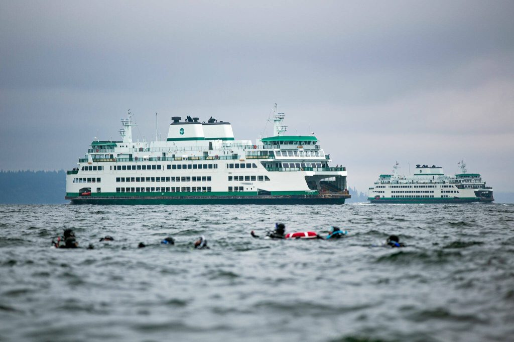
Two ferries out on the water, with swimmers in the foreground. Photo courtesy of a friend, used with permission.
Class topic: MATH& 146, Section 4.4 — contingency tables, marginal and conditional distributions, and Simpson’s paradox.
A month ago I checked a hunch: on summer afternoons, the big boat on my route seems to be the late one. The records agreed. From 2021 to 2025, the 144-car boats left more than 10 minutes late on 39% of summer afternoon sailings. The smaller boats did on 30%.
But I left a warning in that post. The two kinds of boat didn’t run the same weeks. If the big boats happened to work the busiest weeks, they’d look late even if they weren’t any slower. This summer the route was busier than ever: more than 400,000 riders in August 2026, per the Whidbey News-Times. Busy weeks matter.
My class just covered a trap called Simpson’s paradox: a comparison that points one way overall and flips when you split the data into fair groups. So I asked: is the big ferry really late, or did it just work the busy weeks?
Where the numbers come from
Same source as before: Washington State Ferries’ public dashboard, which records how many minutes late every sailing left.1 I matched each sailing to its boat’s car capacity from WSDOT’s vessel pages.2
I kept the same slice as the first post: summer afternoons (June–August, 1 to 7 p.m.), 2021 through 2025, both directions. That’s 10,125 sailings with a recorded delay. This isn’t a sample. It’s every sailing the system recorded, so there’s no margin of error to report.
One limit up front: another 826 afternoon sailings in those summers have no delay and no boat recorded. WSF says very late sailings often go unmatched, so the missing ones are probably some of the latest. I can’t tell which boat ran them, so they’re left out.
What I did in R
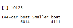
My summer-afternoon sailings in R: how many there are for each boat size.
Show the code
sailings <-read.csv("../2026-09-28-ferry-runs-late/muk-clinton-sailings.csv")# Summer afternoons (June-August, 1-7 pm), 2021-2025, sailings with a recorded delay and a known boataft <-subset(sailings, year %in%2021:2025& month %in%6:8& clock_min >=780& clock_min <1140&!is.na(delay_min) &!is.na(vehicle_capacity))aft$boat <-ifelse(aft$vehicle_capacity ==144, "144-car boat", "Smaller boat")aft$late <-ifelse(aft$delay_min >10, "Late", "On time") # WSF: more than 10 minutes = latenrow(aft)
[1] 10125
Show the code
table(aft$boat)
144-car boat Smaller boat
        6014         4111
The table everything starts from
A contingency table (also called a two-way table) sorts every sailing by two things at once. Here: which size of boat ran it, and whether it left late.
Show the code
tab <-table(aft$boat, aft$late)addmargins(tab) # counts, with totals on the edges
                Late On time   Sum
  144-car boat  2319    3695  6014
  Smaller boat  1226    2885  4111
  Sum           3545    6580 10125
Show the code
round(prop.table(tab, margin =1), 3) # share late WITHIN each boat size
                Late On time
  144-car boat 0.386   0.614
  Smaller boat 0.298   0.702
The totals on the edges are the marginal distributions: each variable on its own. For example, 3,545 of the 10,125 sailings were late, about 35%.
To compare the boats I need conditional distributions: the late share within each boat size. Counts alone mislead here, because the big boats ran more sailings. Within each row:
144-car boats: 2,319 late out of 6,014, or 38.6%
Smaller boats: 1,226 late out of 4,111, or 29.8%
That’s a gap of about 9 percentage points. Now the question is whether it survives a fair comparison.
The suspect: the big boats worked more Augusts
A lurking variable is something that isn’t in my comparison but affects both sides of it. For the boats, the obvious suspect is when each one ran. Here’s how each boat size’s sailings were spread across the summer:
Show the code
round(prop.table(table(aft$boat, aft$month), margin =1), 3) # share of each boat's sailings by month
round(prop.table(table(aft$month, aft$late), margin =1), 3) # share late in each month
     Late On time
  6 0.261   0.739
  7 0.394   0.606
  8 0.395   0.605
That’s lopsided. 41% of the big boats’ sailings were in August, against 23% for the smaller boats. In August 2022 and August 2023, only 144-car boats ran the route in the afternoon. The smaller boats did most of their work in June, the calmest month: 26% of June sailings were late, against about 39% in both July and August.
So the big boats did work more of the busy weeks. That’s exactly the setup where Simpson’s paradox can happen.
Splitting the data every way I could
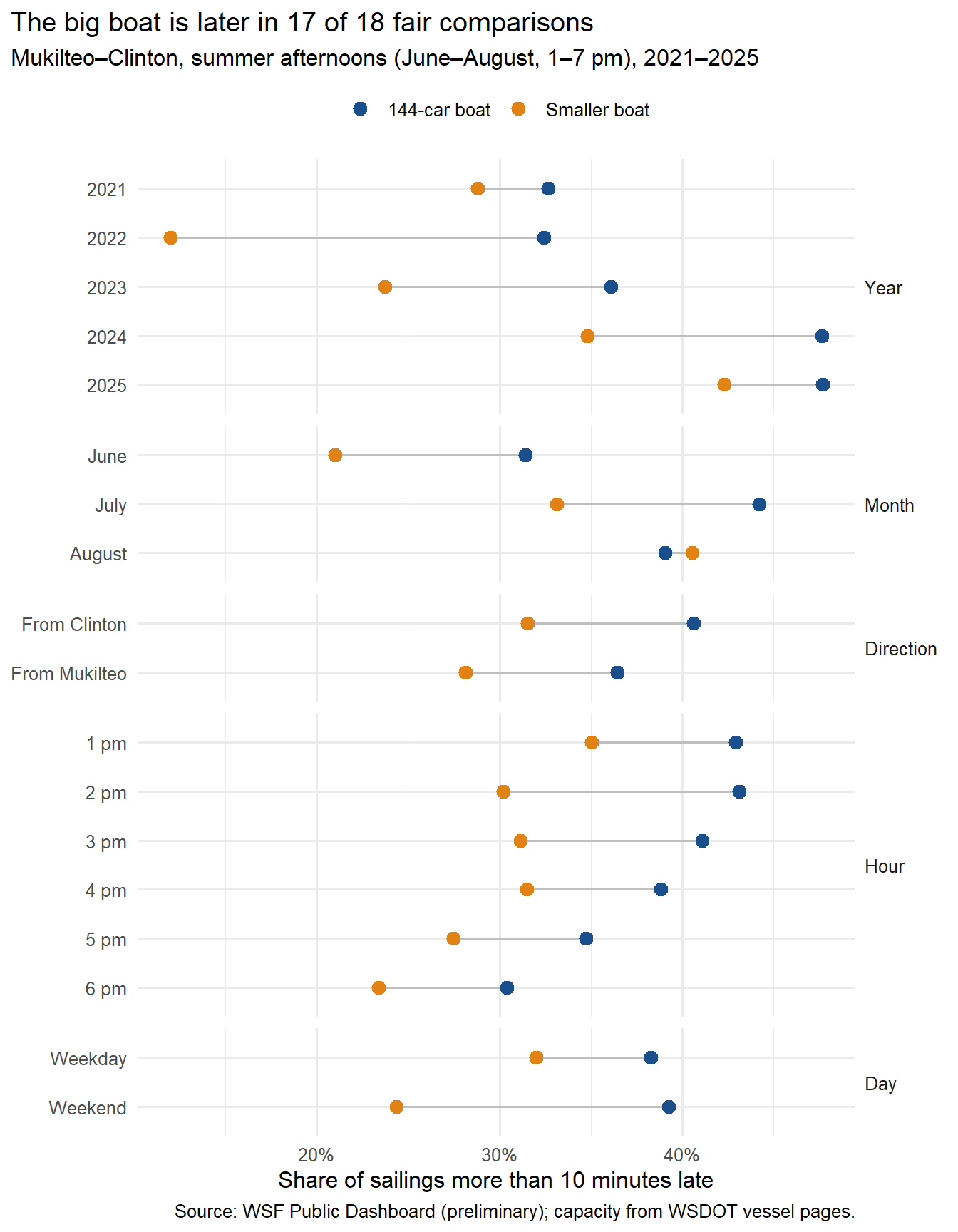
If the gap is only about the calendar, it should shrink or flip once I compare the boats within the same year, the same month, the same direction, the same hour and the same kind of day. Each row in the chart below is one fair group.
Show the code
library(ggplot2)aft$is_late <- aft$late =="Late"aft$hour <-paste0(aft$clock_min %/%60-12, " pm")aft$day_type <-ifelse(aft$weekday %in%c("Saturday", "Sunday"), "Weekend", "Weekday")aft$month_name <-factor(month.name[aft$month], levels = month.name[6:8])splits <-c(Year ="year", Month ="month_name", Direction ="direction",Hour ="hour", Day ="day_type")rows <-list()for (s innames(splits)) { g <-aggregate(aft$is_late, by =list(group = aft[[splits[s]]], boat = aft$boat), FUN = mean) g$split <- s rows[[s]] <- g}by_group <-do.call(rbind, rows)names(by_group)[3] <-"late_share"by_group$group <-factor(by_group$group, levels =rev(unique(by_group$group)))by_group$split <-factor(by_group$split, levels =names(splits))ggplot(by_group, aes(x = late_share, y = group, colour = boat)) +geom_line(aes(group = group), colour ="grey75") +geom_point(size =3) +facet_grid(split ~ ., scales ="free_y", space ="free_y") +scale_colour_manual(values =c("144-car boat"="#1a4f8b", "Smaller boat"="#e08214"), name =NULL) +scale_x_continuous(labels =function(x) paste0(round(100* x), "%")) +labs(x ="Share of sailings more than 10 minutes late", y =NULL,title ="The big boat is later in 17 of 18 fair comparisons",subtitle ="Mukilteo–Clinton, summer afternoons (June–August, 1–7 pm), 2021–2025",caption ="Source: WSF Public Dashboard (preliminary); capacity from WSDOT vessel pages.") +theme_minimal(base_size =12) +theme(plot.title.position ="plot", legend.position ="top",strip.text.y =element_text(angle =0, hjust =0))
The gap doesn’t flip. In every year, both directions, every hour and both kinds of day, the 144-car boats were late more often. The gap gets smaller in some groups (4 points in 2021, 5 points in 2025) and bigger in others (20 points in 2022). But the big boat is on the late side every time, except one.
The paradox hiding inside August
The one exception is August. Across all five Augusts, the smaller boats were late slightly more often: 40.5% against 39.1%.
But look at which Augusts. The smaller boats only ran in August 2021, 2024 and 2025, and 2024 and 2025 were the two latest summers in the data. The big boats ran every August, including 2022 and 2023, when afternoons were calmer. So in August, the smaller boats are the ones that worked the worse weeks.
Show the code
aug <-subset(aft, month ==8)round(tapply(aug$is_late, aug$boat, mean), 3) # all five Augusts
144-car boat Smaller boat
       0.391        0.405
Show the code
aug_shared <-subset(aug, year %in%c(2021, 2024, 2025)) # only the Augusts both sizes ranround(tapply(aug_shared$is_late, aug_shared$boat, mean), 3)
144-car boat Smaller boat
       0.419        0.405
Compare only the Augusts when both sizes ran, and the big boat is the later one again: 41.9% against 40.5%.
That’s Simpson’s paradox, on a small scale. The August result flipped because the two groups were spread across different years. It just turned up in the opposite place from where I expected. I went looking for the calendar to explain away the big boat’s delays, and instead it was hiding a small-boat delay.
How much of the gap is the calendar?
One more way to ask the question: what if the big boats had worked exactly the same weeks as the smaller boats? I can work that out with a weighted average. Take the big boats’ late share in each month of each year, then weight each one by how much of the smaller boats’ work fell in that month.
Show the code
aft$year_month <-paste(aft$year, aft$month)small <- aft$boat =="Smaller boat"small_mix <-prop.table(table(aft$year_month[small])) # smaller boats' calendarbig_rate <-tapply(aft$is_late[!small], aft$year_month[!small], mean) # big boats' late share each monthbig_on_small_calendar <-sum(small_mix * big_rate[names(small_mix)])round(c(big_on_small_calendar = big_on_small_calendar,smaller_boats =mean(aft$is_late[small])), 3)
big_on_small_calendar         smaller_boats
                0.379                 0.298
On the smaller boats’ calendar, the big boats would have been late 37.9% of the time, against 29.8% for the smaller boats. The gap shrinks from 8.7 points to 8.1. So the calendar explains less than one point of it. The big boats really did leave late more often.
Is it the size, or the particular boats?
“Smaller boat” is really a handful of specific boats. Splitting by name:
Show the code
by_vessel <-aggregate(is_late ~ vessel + vehicle_capacity, data = aft, FUN = mean)by_vessel$sailings <-as.vector(table(aft$vessel)[by_vessel$vessel])by_vessel$is_late <-round(by_vessel$is_late, 3)by_vessel[order(-by_vessel$vehicle_capacity, -by_vessel$is_late), ]
The three 144-car boats all land between 38% and 39%. The smaller ones are all over the place. The Chelan carries 124 cars, and it was late as often as the big boats (38.5%, but over only 403 sailings). The Kitsap did most of the smaller-boat work and was late 31.5% of the time. The Issaquah ran only 364 afternoon sailings, in 2022–2023, and was late just 13.7% of the time. The 90-car Sealth, filling in during 2024, was late 25.7% of the time.
The Issaquah’s low number pulls the smaller-boat average down a little. Leave it out and the smaller boats come in at 31.4%, still well below the big boats’ 38.6%. Still, with so few boats, I can’t fully separate “big” from “these particular boats.”
How confident can I be?
No paradox in the main result. The big boats were later overall, later in 17 of 18 fair groups, and later after evening out the calendar. That’s about as solid as a comparison of two groups gets without an experiment.
This shows a pattern, not a cause. WSF chooses which boat runs when. The choice isn’t random, so something I haven’t split by (crew, maintenance, which boat runs on the worst days) could still be part of it. A truly fair test would assign boats at random, and no one is going to do that with a ferry route.
The boats share delays. The two boats take turns at the same docks, so one boat’s delay can spill into the next sailing. I watched this from the deck in the first post, and the last post found that the previous crossing matters a lot. If big-boat delays spill onto the small boat, the real gap could be even bigger than it looks here.
Missing sailings. 826 sailings with no delay and no boat recorded are left out. If they were mostly late big-boat trips, or mostly late small-boat trips, the gap would move.
One route, five summers of afternoons. Mornings, winters and other routes could look different.
The class words for what I found
Class term
In this post
Contingency table
Every sailing sorted by boat size (rows) and late or on time (columns)
Marginal distribution
The table’s edges: 35% of all 10,125 sailings were late
Conditional distribution
The late share within each boat size: 38.6% vs. 29.8%
Lurking variable
When each boat ran: 41% of big-boat sailings were in August vs. 23% for the smaller boats. Evening out the calendar shrinks the gap only from 8.7 to 8.1 points
Simpson’s paradox
In August overall, the smaller boats look later (40.5% vs. 39.1%). Compare only the Augusts both ran, and the big boat is later (41.9% vs. 40.5%)
Association
Boat size and lateness are linked in nearly every group, but that alone doesn’t prove the size causes it
The Tokitae, one of the 144-car boats, crossing between Whidbey Island and Mukilteo in March 2023. Photo: Timothy A. Gonsalves, CC BY-SA 4.0, via Wikimedia Commons.
What I’ll remember from the dock
Do I notice which boat is running? Yes and no. I don’t know the boats by name. But you can tell big from small as one comes in: the big boat has an extra top deck, and the small boat doesn’t.
When I see the small boat coming in, I expect it to unload faster, load faster and leave sooner. I don’t know the actual time each boat spends at the dock. Just from watching, though, I’d say with some confidence that the small boat spends less time there than the big one.
I like riding the big boats more. The small boat has some semi-covered outside seating, which is nice. Sitting inside, there’s no real difference.
So why would the big boat run late more often? My theory is that the small things add up. On a bigger boat, walk-ons may have a longer walk on and off. Drivers have farther to go from the top deck back down to their cars. There’s an extra deck to sweep and check every trip, along with all the bathrooms, for anyone who stayed aboard. That’s 30 seconds here, 30 seconds there, a minute or two for a full sweep. Over every loading and unloading, it adds up. Now and then the crew is also training someone or running a drill, though that’s rare. That’s my guess from the dock. The data in this post can’t show it.
Since we moved here in ’96, the terminals have been upgraded and torn down and rebuilt. There are new systems, new ramps and bigger car lots, and the boats have changed too. My sense is that every new or bigger system brings little intricacies nobody plans for, and each one can add time.
Loading isn’t the same on both sides either. At Clinton there are usually one or two waves of walk-ons: one before the cars load and one after. When the boat is running behind, they send everyone in a single wave after the cars. At Mukilteo there’s the sky bridge, so walk-ons board whenever the door opens.
That’s a lot of variables. If I wanted to settle “size or these particular boats,” I’d stand at the dock with a stopwatch. How long does a full boat take to unload, and an empty one to load, big boat versus small? My class calls that an observational study: I’d measure what happens without changing anything. It still couldn’t prove the size causes the difference, but it would show where the minutes go.
Sources:WSF Public Dashboard, On-Time Performance by sailing, Mukilteo–Clinton, summers 2021–2025 (preliminary), exported Sept. 26, 2026 · WSDOT VesselWatch vessel pages, pulled Sept. 26, 2026 · Whidbey News-Times, Sept. 15, 2026. Photos: credited above. Data file:muk-clinton-sailings.csv in the earlier post’s folder, built by its prepare-data.R from the dashboard exports in data/raw/.
Washington State Ferries, WSF Public Dashboard (Tableau Public), On-Time Performance by sailing, Mukilteo–Clinton, data through June 30, 2026, labeled preliminary. Exported Sept. 26, 2026.↩︎